Using Gradient Boosting Machines to Model Risk Premiums

This is a project I did for a swedish insurance company, with the goal to make their pricing strategy for a home insurance product more competitive using machine learning. As the insurance industry is highly data driven it is no surprise that machine learning (ML) has made its way into the industry. While GLMs are still the comfort zone of most actuaries, we have in recent years seen a surge in machine learning algorithms. This study puts focus on developing and evaluating three tree-based machine learning models, starting from simple decision trees and working up to the more advanced ensemble methods random forests and gradient boosting machines.

Insurance Pricing Fundamentals

First, it is important to understand why setting a premium that rightfully corresponds to the risk of the customer is so crucial for the insurer. We will highlight this with a simple example. Assume two insurers, A and B, exist and A has a low premium relative to the risk of loss, while B has an adequate premium in relation to the risk. In this scenario, a high risk customers would opt for A since their premium is relatively low compared to B, thus A would attract high risk customers and in effect see their margins being eaten up. On the contrary, if A’s premiums are too high they would not attract any profitable customers and still lose money. In the light of this simple example, we see why a competitive pricing strategy is paramount. Perhaps, the most common pricing strategy is the frequency-severity strategy. In the frequency-severity model we assume that two factors will influence the risk of a customer:

• Frequency (F) - number of claims per exposure time
• Severity (S) - average loss per claim

where exposure is the time for which a risk is insured. Now, assume that an insurer has a total loss of \(L\) spread out over \(N\) claims and an exposure \(e\). Then the effective, or technical premium would be:

\[\begin{equation} \tau = \mathbb{E}\left(\frac{L}{e}\right) = \mathbb{E}\left(\frac{L}{N} \lvert N >0\right) \times \mathbb{E}\left(\frac{N}{e}\right) = \mathbb{E}\left(S\right) \times \mathbb{E}\left(F\right) \end{equation}\]

Where we have assumed independence between the frequency and severity. By this reduction, insurance pricing becomes a problem of predicting $S$ and $F$. Be that as it may, in this case we will restrict our study to the frequency.

Modelling the Frequency Using Decision Trees

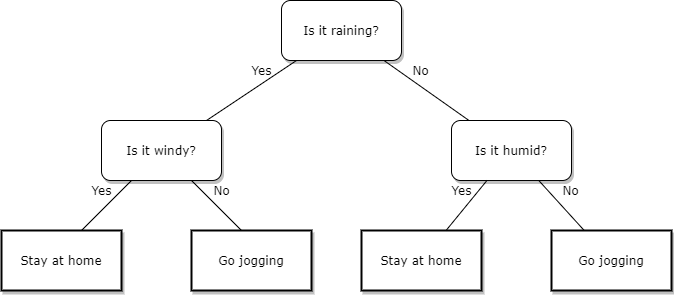
One common type of ML model is the decision tree, introduced by Breiman et al. in 1984, which is a very intuitive and natural model for us humans as it in a way mimics the way we make decisions. A decision tree divides the predictor space into a number of exhaustive and non-overlapping subsets, with a fitted response for each subset. As such, using a indicator function each input can be mapped to a response depending on what subset the input lands in. A very simple example of a decision tree can be seen in the figure below:

The most common way to train a decision tree is through the CART algorithm which essentially minimizes two terms when dividing the predictor space \(R = \cup_{j=1}^{J}R_j\):

\begin{equation} \sum_{j=1}^{J}\left[\sum_{x_i\in R_j} \mathcal{L}(y_i, \hat{y_{R_j}})\right] + \text{cp}\cdot J\sum_{x_i \in R}\mathcal{L}(y_i, \hat{y}_R) \end{equation}

where the first term ensures a good fit and the second reduces overfitting according to the constant cp, with cp = 1 resulting in a tree without splits and cp = 0 a maximally deep tree. The parameter cp is most commonly done through cross validation. Moreover, the loss function can be chosen depending on the context, in this case we are dealing with Poisson distributed claims data, so the Poisson deviance is appropriate.

Ensemble Methods

There are obvious advantages of decision trees, such as their interpretability and the fact that they can combine both continuous and discrete data. However, they also have their limitations. For one, single decision trees tend to have a rather high variance and can be very sensitive to the training data. In order to counteract this shortcoming, so called ensemble methods can be used, in which multiple weak models are aggregated into a more powerful predictor. I focused on the gradient boosting machine in this work as it has received the most praise for its predicitve performance.

J. Friedman introduced gradient boosting in his 1999 paper. The general problem of predictive modelling is, as we now know, to find a function $f(\bm{x})$ to predict a response variable y from a set of explanatory variables x, which minimises some loss function \(\mathcal{L}(f(x), y)\). Gradient boosting is considered a gradient descent algorithm, meaning it relies on iterative tuning of parameters in order to achieve the minimium of a specified loss function.

In boosting, \(f(x)\) is estimated by an expansion of the form: \begin{equation} \hat{f}(x) = \sum_{m=0}^M \beta_m h(x, a_m)
\end{equation}

where the base learners \(h(x, a_m)\) are usually chosen to be simple functions with parameters a. Both a and \(\beta\) are fitted to the training data in a step-wise manner.

The Data

Now, as insurace claims are rather rare per exposure the data is very skewed:

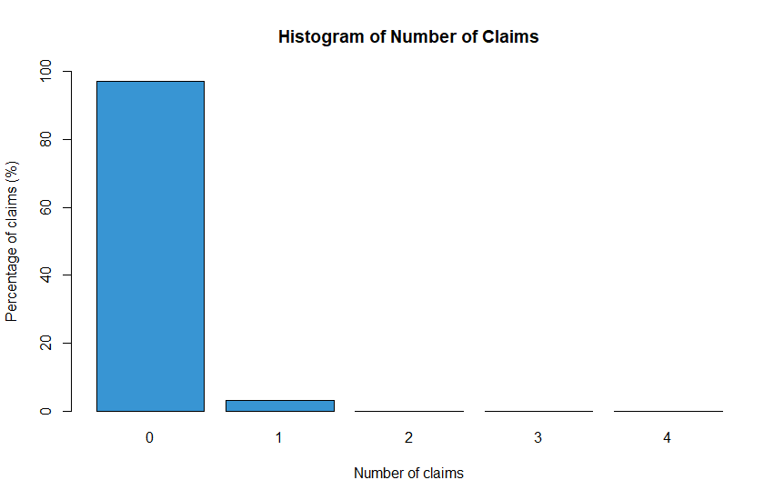
This can become a problem as the model might learn to only predict a frequency of zero, however we also want to capture the attributes of those customers that do not have any claims. One approach to this problem is to view the task as a binary classification task at first, where zero claims and > 0 claims are seperated. Subsequently, a regression model can be fit on the > 0 class. In my work, I decided to downsample the data according to the minority class as the amount of data was very large. I also investigated a technique called SMOTE (https://arxiv.org/pdf/1106.1813.pdf) for upsampling the minority class.

Outliers

For the all-risk cover, only claims that have a severity of 50,000SEK or less are covered by the insurance. Therefore, all values above 50,000 were set to 50,000. Moreover, there were several faulty observations, such as negative claims, which were omitted.

Uncertain data

In paying a claim there are three important quantities, the amount incurred but not reported (IBNR), the amount reported but not settled (RBNS) and the amount that has been paid to the customer. The insurance company will reserve money to cover the RBNS and the IBNR, and after the claim has been made by the insured this reserve will start being paid out to the customer until the claim is closed. There is a certain uncertainty in the RBNS, which could be an issue. Therefore the data was truncated so that the fraction of RBNS was relatively low.

Missing values

Rows containing missing values where removed only if they were missing for an important feature or for one of the response variables, as most model implementations cannot deal with missing values. This of course reduces the amount of data, but given the size of the data set this is not a great loss. After the data preparation, around 140,000 observations were left.

Modelling

I decided to keep it relatively simple in this project and used only 4 explanatory variables:

Variable Name	Description
NO_CLAIM_NOT_NULL	Number of claims
EXP_COV	Exposure measured in years
AGE_INSUR_PERS	Age of the insurance taker
NO_INSUR	Number of people in the insured property
ACCOM_TYPE_NAME	Type of property
LIVE_AREA	The total surface area of the property

With these features, I trained a simple decision tree model and a gradient boosting machine using the CART algorithm. Moreover, I ran a extensive cross validation scheme to optimize the hyperparameters of the models. Using an average over the cross validation folds I obtained the optimal models that I finally tested against each other.

Results

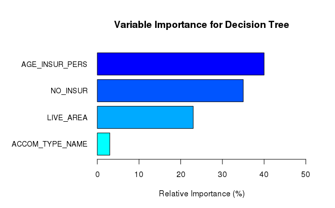
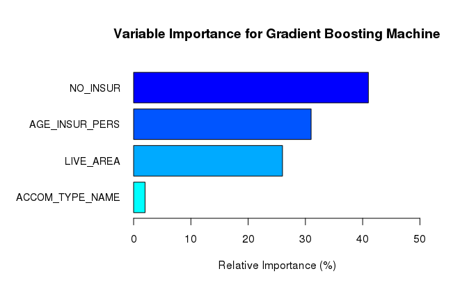
Firstly, I evaluated the variable importance of the independent variables for each of the two models using the average of the optimal parameters found using the cross-validation scheme. Below are the results for each model.

Secondly, as mentioned above, I averaged the Poisson deviance over 6 cross validation folds to see which model had the best performance:

Fold	Decision tree	Gradient boosting machine
Average deviance	0.255	0.253

Conlcusions

Variable Importance

Firstly, neither model considers the accommodation type as an important feature, having the lowest relative importance for both models. Secondly, both models consider the age of the insured to be an important variable. Thirdly, regarding the number of people in the household, both the decision tree and the gradient boosting machine agree that this variable is relatively important.

Deviance

The cross-validation results show that the gradient boosting machine on average has the best predicitve performance. Even though the difference in average deviance between the two models looks miniscule, a slight improvement could lead to large business value. Although the simple decision tree has worse performance than the gradient boosting machine, it has the advantage of being simple, very fast to train and easily interpretable. According to the European Union General Data Protection Regulation (GDPR), in the context of automated decision-making, the data subject should have the right to obtain an explanation of the decision reached, therefore it is important to be able to understand, interpret and evaluate the models that are built.

For a full report and code for this project please refer to this link.