Convolutional Neural Network from Scratch
Recently I built, trained and optimized a convolutional neural network (CNN) from scratch using Python with Numpy. In this post I will guide you through my work by explaining the architecture of CNNs, how I trained the CNN, and finally how I evaluated its performance. The aim for my CNN was to predict the country of origin for a given family name, i.e. we have a multi-class classification problem at hand. The code for this project can be found at: Link to code
Examining the Data and Encoding the Input
The Data Set
Before I get into details on CNNs and network optimization, let us have a look at the data set. Below is a sample from the data set:
| Family Name | Country | Country Label |
|---|---|---|
| Parkinson | England | 5 |
| Wang | China | 2 |
| Blumenthal | Germany | 7 |
This is what the raw data will look like. Note how each country has a unique label and when we train the network we will train it on the country labels instead of the country name. Let’s look at the distribution of classes in the data set:
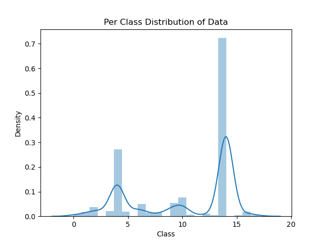
Clearly the data set is not balanced, how this affects the network’s performance and how it can be mitigated, is something we will come back to later.
Encoding the Input
Now, we cannot train a CNN on the family names in their raw form, we have to convert into a format that is compatible with CNNs. For this project, I used one hot encoding on the character level, i.e. each character is represented by a vector with fixed length, and all zeros but in one position. The length of each character vector will be the size of the vocabulary, let’s call this \(V\), that is the number of unique characters in our data set. This is easier understood with an example. Take the name Wang, and let’s for simplicity assume we have a vocabulary of size 4, containing only the characters in Wang. We can then map each letter to a unit vector, for example encoding the letters \(\{w, a, n, g\}\) in alphabetical order:
\begin{equation} \text{w} \rightarrow \begin{bmatrix}0 & 0 & 0 & 1\end{bmatrix}^T \end{equation} \begin{equation} \text{a} \rightarrow \begin{bmatrix}1 & 0 & 0 & 0\end{bmatrix}^T \end{equation} \begin{equation} \vdots \end{equation}
etc…
Thus, a word of length \(M\) will be represented by a \(M \times V\) matrix. Using our example:
\[\text{wang} \rightarrow \begin{bmatrix}0 & 1 & 0 & 0 \\ 0 & 0 & 0 & 1 \\ 0 & 0 & 1 & 0 \\ 1 & 0 & 0 & 0\end{bmatrix}\]In our case, we will have names of varying length, therefore we will use a fixed matrix dimension of \(M_{\text{max}} \times V\), where \(M_{\text{max}}\) is the length of the longest word in our vocabulary. If a word has a length smaller than \(M_{\text{max}}\), the remaining columns will just be zero vectors.
Now, as some of you might know a CNN takes a matrix as input, and so far we have represented one word with a matrix, hence if we have a whole set of words this would be represented by a 3 dimensional tensor, which is not what we want to have. To transform our input to a matrix, we will flatten the word matrices into vectors. Where the flattening operation on a matrix is defined by:
\[A = \begin{bmatrix}a & b \\ c & d\end{bmatrix} \rightarrow \text{flatten}(A) = \begin{bmatrix}a \\ c \\b \\ d\end{bmatrix}\]With this encoding, the whole data set can be represented by one matrix \(X\) of size \((M_{\text{max}} \times V) \times N\), where \(N\) is the number of names in the data set. Similarly, we encode the country label using one hot encoding and concatenate all the country labels into a matrix \(Y\) of size \(L \times N\) where \(L\) is the number of unique labels in the data set.
Dealing With Unbalanced Data
There are a few ways in which one can mitigate the problem of unbalanced classes in a classification setting. Perhaps the most straight forward and simple way is to downsample the data according to the number of data points in the minority class, that is, if the minority class contains \(n\) data points, we randomly sample \(n\) rows from all classes and use this as our training data. It may seem that with this approach, we are discarding a lot of data, however, if one performs this sampling each epoch and trains the network for enough epochs, the network will have been trained on most of the original data; we are just ensuring that each time the model is shown a set of data points, the corresponding classes are uniformly distributed.
An Overview of CNNs
CNNs suit themselves best to solving problems where the input data is in the form of a tensor, which is one of the reasons they have found a lot of popularity in tasks where the input consists of visualy imagery. Moreover, CNNs are shift invariant which in non-technical terms means that it does not matter where, in say for example an image, a feauture is, the network will still recognize this as the same feature. This is an especially desired property in image classification, but perhaps not so relevant in the task we have at hand.
CNN Architecture
CNNs consists of three types of layers: Convolutional layers, pooling layers and fully connected layers. I will not go into great technical detail of the different layers as there already is a plethora of great resources to read up on the specifics of CNNs, instead I will just offer a brief overview. Firstly, the convolutional layers consist of a number of filters, and perform convolutions of the input tensor and these filters, producing a 2d activation map. Thus the network learns filters that activate when stimulated by certain features in the input. Secondly, the pooling layers act as a form of regularization by progressively decreasing the size of the representations, the number of parameters, the memory usage and hence also helps in mitigating overfitting. Finally, the cascade of pooling and convolutional layers is fed into a fully connected layer that computes the final activations, and in our case, comptues the probabilities of the diferent classes through a softmax function. For a illustration of a typical CNN architecture, see the image below.

Training the CNN
Loss Function
Before we try can train the CNN, we have to decide on a loss function. In this project I went for the cross entropy loss, defined as:
\begin{equation} L = -\frac{1}{|X|} \sum_{x,y \in X, Y}y\log{p} \end{equation} where \(p\) is the vector of class probabilities resulting from a forward pass through the entire network, and \(y\) is the one-hot encoding of the label as described in the section above.
Forward-pass
The forward pass of the CNN is quite simple: Firstly we convolve the input tensor through a set of convolutional layers \(F_i\), \(i = 1,2,3,...\), and secondly we multiply the output from the convolutional layers with a weight matrix, \(W\):
set x <- X
for F_i in Filters do:
    x = max(0, X * F_i)

s = W @ flatten(x)
p = Softmax(s)
where * denotes the convolution operation and @ normal matrix multiplication. I will cover how I implemented the convolution operation in the final section. Once we have the probabilites p, the predicted class and loss can easily be calcluated and used in the backward pass. Note that I in this implementation have ignored the bias term as well as pooling layers.
Backward-pass
Typically a CNN is trained using normal backpropagation, and here, in order to propagate the error, one has to compute the gradients with respect to both the filters and the weights connecting the fully connected layer (note that if one uses bias in the fully connected layer, of course the gradient with respect to this bias also has to be computed). The gradients are computed analytically as a numerical implementation would be far slower, this can be quite cumbersome but it is definetly worth it in terms of efficiency gains. I present a full derivation of the gradients in the final section, for those who are interested.
Optimization Scheme
There are many options when it comes to how exactly the loss surface is traversed to find minimas of the loss function, one typically controls this process through the learning rate \(\eta\), momentum, mini-batch training etc… I decided to use momentum and perform the gradient descent in mini-batches, i.e. to divide the input data set into smaller size batches and perform backpropagtion on these. With these choices, there are effectively five hyper-parameters: \(\eta\), the mini-batch size, the momentum term (\(\rho\)), the number of filters per layer and the filter widths. As always, these parameters are best selected through a grid search.
The Influence of Unbalanced Data
To investigate whether the very skewed original data set had any effect on the network’s performance, I compared two models: One trained on the original data set, and one trained on a data set that I had downsampled prior to training. Here one has to be careful as to what metrics to use when comparing the two models, when dealing with unbalanced data a single accuracy for the whole data set might not be the best option as a model that solely predicts the majority class will have a high accuracy while not being a good model. In this project I opted for confusion matrices and F-score as my primary evaluation metric as these give a more complete picture of the model performance. More on this later.
Results of Training
I trained the network through 20 000 update steps, one update step being one update of the gradients, and the tracked the validation and training loss and accuracy every 50th update step. Moreover, I utilized early stopping to ensure that the model corresponding to the validation loss minimum is saved. Using 2 convolutional layers with 50 filters each, a learning rate of 0.01, momentum term of 0.9 and batch size of 100, the final validation accuracy was 53% on the balanced data, and 47% on the unbalanced data. In the figure below the loss is plotted per 10 update steps.
Evaluating the Network’s Performance
To Evaluate the CNN I generated confusion matrices and calculated the F-score for both the balanced and unbalanced data sets.
Final Remarks
Appendix
Convolution using Matrix Multiplication
To make the back-propagation algorithm transparent and relatively efficient(as I ran this on CPU not a GPU and to take computational advantage of the sparse input data) we will set up the convolutions per-formed as matrix multiplications. In the following I will show how you can set up the appropriate matrix based on the entries of the applied for a small example. Let X be a 4 x 4 input matrix and F be a 4 x 2 filter:
\(X = \begin{bmatrix}X_{11} & X_{12} & X_{13} & X_{14} \\ X_{21} & X_{22} & X_{23} & X_{24} \\ X_{31} & X_{32} & X_{33} & X_{34} \\ X_{41} & X_{42} & X_{43} & X_{44}\end{bmatrix}\), \(F = \begin{bmatrix}F_{11} & F_{12} \\ F_{21} & F_{22} \\ F_{31} & F_{32} \\ F_{41} & F_{42}\end{bmatrix}\)
When we convolve X with F (stride 1 and no zero-padding), the output vector has size 3 x 1:
\[s = X * F \implies s = M^{filter}_{F,4} @ flatten(X)\]where \(M^{filter}_{F,4}\) is 3 x 16 and the subscript 4 denotes the number of rows in X. The latter is needed to specify the number of columns in \(M^{filter}_{F,4}\) given the width of F. Thus,
\[M^{filter}_{F,4} = \begin{bmatrix}F_{11} & F_{21} & F_{31} & F_{41} & F_{12} & F_{22} & F_{32} & F_{42} & 0 & 0 & 0 & 0 & 0 & 0 & 0 & 0\\ 0 & 0 & 0 & F_{11} & F_{21} & F_{31} & F_{41} & F_{12} & F_{22} & F_{32} & F_{42} & 0 & 0 & 0 & 0 \\ 0 & 0 & 0 & 0 & 0 & 0 & 0 & 0 & F_{11} & F_{21} & F_{31} & F_{41} & F_{12} & F_{22} & F_{32} & F_{42} \end{bmatrix}\]which, using some notation, can be simplified to:
\[M^{filter}_{F,4} = \begin{bmatrix}\leftarrow v^T \rightarrow & 0_4^T & 0_4^T \\ 0_4^T & \leftarrow v^T \rightarrow & 0_4^T \\ 0_4^T & 0_4^T & \leftarrow v^T \rightarrow \end{bmatrix}\]where \(v^T = flatten(F)\) and \(0_4^T\) is a row vector of 4 zeros. This pattern can then be extended a \(X\) with arbitrary dimensions.